
Gamma Distribution Function
The gamma distribution is a two-parameter family of continuous probability distributions. While it is used rarely in its raw form but other popularly used distributions like exponential, chi-squared, erlang distributions are special cases of the gamma distribution. The gamma distribution can be parameterized in terms of a shape parameter α=kα=k and an inverse scale parameter β=1/θβ=1/θ, called a rate parameter., the symbol Γ(n)Γ(n) is the gamma function and is defined as (n−1)!(n−1)! :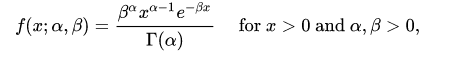
A typical gamma distribution looks like: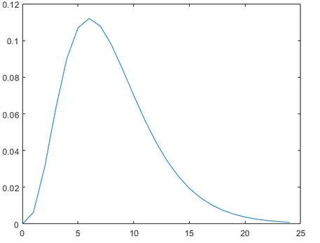
Gamma Distribution in Python
You can generate a gamma distributed random variable using scipy.stats module’s gamma.rvs() method which takes shape parameter aa as its argument. When aa is an integer, gamma reduces to the Erlang distribution, and when a=1a=1 to the exponential distribution. To shift distribution use the loc argument, to scale use scale argument, size decides the number of random variates in the distribution. If you want to maintain reproducibility, include a random_state argument assigned to a number.
from scipy.stats import gamma
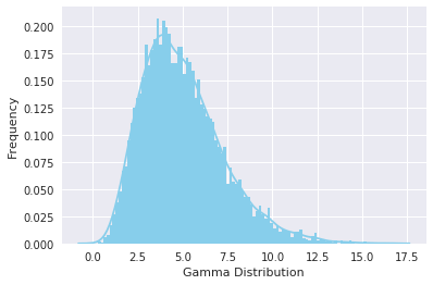
data_gamma = gamma.rvs(a=5, size=10000)
You can visualize the distribution just like you did with the uniform distribution, using seaborn’s distplot functions. The meaning of the arguments remains the same as explained in the uniform distribution section.
ax = sns.distplot(data_gamma,
                  kde=True,
                  bins=100,
                  color='skyblue',
                  hist_kws={"linewidth": 15,'alpha':1})
ax.set(xlabel='Gamma Distribution', ylabel='Frequency')
[Text(0,0.5,u'Frequency'), Text(0.5,0,u'Gamma Distribution')]
Exponential Distribution Function
The exponential distribution describes the time between events in a Poisson point process, i.e., a process in which events occur continuously and independently at a constant average rate. It has a parameter λλ called rate parameter, and its equation is described as :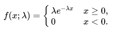
A decreasing exponential distribution looks like :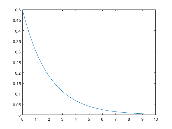
Exponential Distribution in Python
You can generate an exponentially distributed random variable using scipy.stats module’s expon.rvs() method which takes shape parameter scale as its argument which is nothing but 1/lambda in the equation. To shift distribution use the loc argument, size decides the number of random variates in the distribution. If you want to maintain reproducibility, include a random_state argument assigned to a number.
from scipy.stats import expon
data_expon = expon.rvs(scale=1,loc=0,size=1000)
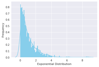
Again visualizing the distribution with seaborn yields the curve shown below:
ax = sns.distplot(data_expon,
                  kde=True,
                  bins=100,
                  color='skyblue',
                  hist_kws={"linewidth": 15,'alpha':1})
ax.set(xlabel='Exponential Distribution', ylabel='Frequency')
[Text(0,0.5,u'Frequency'), Text(0.5,0,u'Exponential Distribution')]
Poisson Distribution
Poisson random variable is typically used to model the number of times an event happened in a time interval. For example, the number of users visited on a website in an interval can be thought of a Poisson process. Poisson distribution is described in terms of the rate (μμ) at which the events happen. An event can occur 0, 1, 2, … times in an interval. The average number of events in an interval is designated λλ (lambda). Lambda is the event rate, also called the rate parameter. The probability of observing kk events in an interval is given by the equation: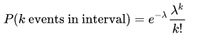
Note that the normal distribution is a limiting case of Poisson distribution with the parameter λ→∞λ→∞. Also, if the times between random events follow an exponential distribution with rate λλ, then the total number of events in a time period of length tt follows the Poisson distribution with parameter λtλt.
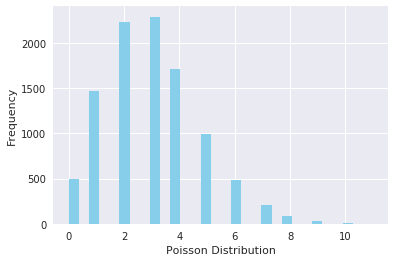
The following figure shows a typical poisson distribution: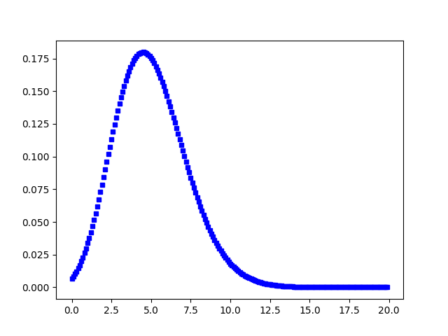
Poisson Distribution in Python
You can generate a poisson distributed discrete random variable using scipy.stats module’s poisson.rvs() method which takes μμ as a shape parameter and is nothing but the λλ in the equation. To shift distribution use the loc parameter. size decides the number of random variates in the distribution. If you want to maintain reproducibility, include a random_state argument assigned to a number.
from scipy.stats import poisson
data_poisson = poisson.rvs(mu=3, size=10000)
You can visualize the distribution just like you did with the uniform distribution, using seaborn’s distplot functions. The meaning of the arguments remains the same.
ax = sns.distplot(data_poisson,
                  bins=30,
                  kde=False,
                  color='skyblue',
                  hist_kws={"linewidth": 15,'alpha':1})
ax.set(xlabel='Poisson Distribution', ylabel='Frequency')
[Text(0,0.5,u'Frequency'), Text(0.5,0,u'Poisson Distribution')]
Binomial Distribution Function
A distribution where only two outcomes are possible, such as success or failure, gain or loss, win or lose and where the probability of success and failure is same for all the trials is called a Binomial Distribution. However, The outcomes need not be equally likely, and each trial is independent of each other. The parameters of a binomial distribution are nn and pp where nn is the total number of trials, and pp is the probability of success in each trial. Its probability distribution function is given by :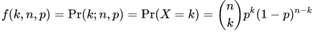
where :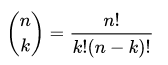
Binomial Distribution in Python
You can generate a binomial distributed discrete random variable using scipy.stats module’s binom.rvs() method which takes nn (number of trials) and pp (probability of success) as shape parameters. To shift distribution use the loc parameter. size decides the number of times to repeat the trials. If you want to maintain reproducibility, include a random_state argument assigned to a number.
from scipy.stats import binom
data_binom = binom.rvs(n=10,p=0.8,size=10000)
Visualizing the distribution you just created using seaborn’s distplot renders the following histogram:
ax = sns.distplot(data_binom,
                  kde=False,
                  color='skyblue',
                  hist_kws={"linewidth": 15,'alpha':1})
ax.set(xlabel='Binomial Distribution', ylabel='Frequency')
[Text(0,0.5,u'Frequency'), Text(0.5,0,u'Binomial Distribution')]
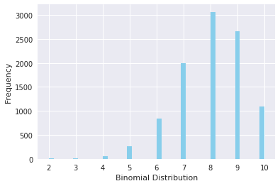
Note that since the probability of success was greater than 0.50.5 the distribution is skewed towards the right side. Also, poisson distribution is a limiting case of a binomial distribution under the following conditions:
- The number of trials is indefinitely large or n→∞n→∞.
- The probability of success for each trial is same and indefinitely small or p→0p→0.
- np=λnp=λ, is finite.
Normal distribution is another limiting form of binomial distribution under the following conditions:
- The number of trials is indefinitely large, n→∞n→∞.
- Both pp and qq are not indefinitely small.
Bernoulli Distribution Function
A Bernoulli distribution has only two possible outcomes, namely 11 (success) and 00 (failure), and a single trial, for example, a coin toss. So the random variable XX which has a Bernoulli distribution can take value 11 with the probability of success, pp, and the value 00 with the probability of failure, qq or 1−p1−p. The probabilities of success and failure need not be equally likely. The Bernoulli distribution is a special case of the binomial distribution where a single trial is conducted (n=1n=1). Its probability mass function is given by:
Bernoulli Distribution in Python
You can generate a bernoulli distributed discrete random variable using scipy.stats module’s bernoulli.rvs() method which takes pp (probability of success) as a shape parameter. To shift distribution use the loc parameter. size decides the number of times to repeat the trials. If you want to maintain reproducibility, include a random_state argument assigned to a number.
from scipy.stats import bernoulli
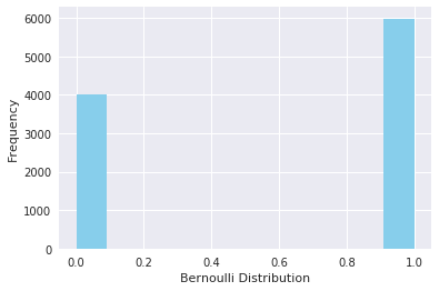
data_bern = bernoulli.rvs(size=10000,p=0.6)
Again visulaizing the distribution, you can observe that you have only two possible outcomes:
ax= sns.distplot(data_bern,
                 kde=False,
                 color="skyblue",
                 hist_kws={"linewidth": 15,'alpha':1})
ax.set(xlabel='Bernoulli Distribution', ylabel='Frequency')
[Text(0,0.5,u'Frequency'), Text(0.5,0,u'Bernoulli Distribution')]
Conclusion
Congrats, you have made it to the end of this tutorial! In this tutorial, you explored some commonly used probability distributions and learned to create and plot them in python. Although there are many other distributions to be explored, this will be sufficient for you to get started. Don’t forget to check out python’s scipy library which has other cool statistical functionalities. Happy exploring!