Skewed Distribution in Python

Find skewness of data in Python using Scipy

we simply use this library byfrom Scipy.stats import skew

Skewness based on its types

There are three types of skewness :

• Normally Distributed: In this, the skewness is always equated to zero.

Skewness=0

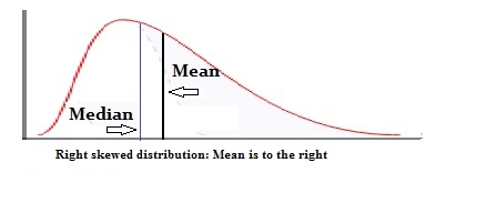
• Positively skewed distribution: In this, A Positively-skewed distribution has a long right tail, that’s why this is also known as right-skewed distribution. the reason behind it, in this value of mode is highest and mean is least which leads to right peak.

Skessness >o

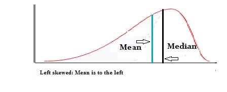
• Negatively skewed distribution: In this, a negatively skewed distribution has a long left tail, that’s why this is also known as left-skewed distribution. the reason behind it, in this value of mode is least and mean is highest just reverse to right-skewed which leads to the left peak.

Skewness<0

The formula to find skewness of data

Skewness =3(Mean- Median)/Standard Deviation

Example: skewness for given data

Input: Any random ten input

from scipy.stats import skew
import numpy as np
x= np.random.normal(0,5,10)
print("X:",x)
print("Skewness for data :",skew(x))

Output:

X: [ 5.51964388 -1.69148439 -5.55162585 -5.6901246   2.38861009  2.73400871
  3.77918369 -2.30759396  3.67021073  1.48142813]
Skewness for data : -0.4625020248485552

---

---

scipy.stats.skewnorm() is a skew-normal continuous random variable. It is inherited from the of generic methods as an instance of the rv_continuous class. It completes the methods with details specific for this particular distribution.

Parameters :

q : lower and upper tail probability
x : quantiles
loc : [optional]location parameter. Default = 0
scale : [optional]scale parameter. Default = 1
size : [tuple of ints, optional] shape or random variates.
moments : [optional] composed of letters [‘mvsk’]; ‘m’ = mean, ‘v’ = variance, ‘s’ = Fisher’s skew and ‘k’ = Fisher’s kurtosis. (default = ‘mv’).

Results : skew-normal continuous random variable

Code #1 : Creating skew-normal continuous random variable

# importing library   from scipy.stats import skewnorm     numargs = skewnorm .numargs  a, b = 4.32, 3.18 rv = skewnorm (a, b)      print ("RV : \n", rv)

Output :

RV : 
 scipy.stats._distn_infrastructure.rv_frozen object at 0x000002A9D843A9C8

Code #2 : skew-normal continuous variates and probability distribution

import numpy as np  quantile = np.arange (0.01, 1, 0.1)    # Random Variates  R = skewnorm.rvs(a, b)  print ("Random Variates : \n", R)    # PDF  R = skewnorm.pdf(a, b, quantile)  print ("\nProbability Distribution : \n", R)

Output :

Random Variates : 
 4.2082825614230845

Probability Distribution : 
 [7.38229165e-05 1.13031801e-04 1.71343310e-04 2.57152477e-04
 3.82094976e-04 5.62094062e-04 8.18660285e-04 1.18047149e-03
 1.68525001e-03 2.38193677e-03]

Code #3 : Graphical Representation.

import numpy as np  import matplotlib.pyplot as plt       distribution = np.linspace(0, np.minimum(rv.dist.b, 3))  print("Distribution : \n", distribution)       plot = plt.plot(distribution, rv.pdf(distribution))

Output :

Distribution : 
 [0.         0.04081633 0.08163265 0.12244898 0.16326531 0.20408163
 0.24489796 0.28571429 0.32653061 0.36734694 0.40816327 0.44897959
 0.48979592 0.53061224 0.57142857 0.6122449  0.65306122 0.69387755
 0.73469388 0.7755102  0.81632653 0.85714286 0.89795918 0.93877551
 0.97959184 1.02040816 1.06122449 1.10204082 1.14285714 1.18367347
 1.2244898  1.26530612 1.30612245 1.34693878 1.3877551  1.42857143
 1.46938776 1.51020408 1.55102041 1.59183673 1.63265306 1.67346939
 1.71428571 1.75510204 1.79591837 1.83673469 1.87755102 1.91836735
 1.95918367 2.        ]
  

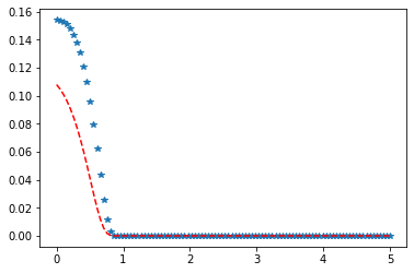
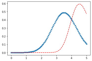
Code #4 : Varying Positional Arguments

import matplotlib.pyplot as plt  import numpy as np       x = np.linspace(0, 5, 100)       # Varying positional arguments  y1 = skewnorm .pdf(x, 1, 3, 5)  y2 = skewnorm .pdf(x, 1, 4, 4)  plt.plot(x, y1, "*", x, y2, "r--")

Output :

---

Left-skewed Levy Distribution in Statistics

scipy.stats.levy_l() is a left-skewed Levy continuous random variable. It is inherited from the of generic methods as an instance of the rv_continuous class. It completes the methods with details specific for this particular distribution.

Parameters :

q : lower and upper tail probability
x : quantiles
loc : [optional]location parameter. Default = 0
scale : [optional]scale parameter. Default = 1
size : [tuple of ints, optional] shape or random variates.
moments : [optional] composed of letters [‘mvsk’]; ‘m’ = mean, ‘v’ = variance, ‘s’ = Fisher’s skew and ‘k’ = Fisher’s kurtosis. (default = ‘mv’).

Results : left-skewed Levy continuous random variable

Code #1 : Creating left-skewed Levy continuous random variable

# importing library   from scipy.stats import levy_l       numargs = levy_l.numargs  a, b = 4.32, 3.18 rv = levy_l(a, b)       print ("RV : \n", rv)

Output :

RV : 
 scipy.stats._distn_infrastructure.rv_frozen object at 0x000002A9D6707508

Code #2 : left-skewed Levy continuous variates and probability distribution

import numpy as np  quantile = np.arange (0.03, 2, 0.21)    # Random Variates  R = levy_l.rvs(a, b)  print ("Random Variates : \n", R)    # PDF  R = levy_l.pdf(a, b, quantile)  print ("\nProbability Distribution : \n", R)

Output :

Random Variates : 
 1.1073459342251062

Probability Distribution : 
 [0. 0. 0. 0. 0. 0. 0. 0. 0. 0.]
 

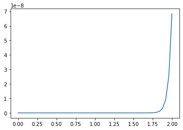
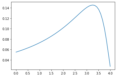
Code #3 : Graphical Representation.

import numpy as np  import matplotlib.pyplot as plt       distribution = np.linspace(0, np.maximum(rv.dist.b, 4))  print("Distribution : \n", distribution)       plot = plt.plot(distribution, rv.pdf(distribution))

Output :

Distribution : 
 [0.         0.08163265 0.16326531 0.24489796 0.32653061 0.40816327
 0.48979592 0.57142857 0.65306122 0.73469388 0.81632653 0.89795918
 0.97959184 1.06122449 1.14285714 1.2244898  1.30612245 1.3877551
 1.46938776 1.55102041 1.63265306 1.71428571 1.79591837 1.87755102
 1.95918367 2.04081633 2.12244898 2.20408163 2.28571429 2.36734694
 2.44897959 2.53061224 2.6122449  2.69387755 2.7755102  2.85714286
 2.93877551 3.02040816 3.10204082 3.18367347 3.26530612 3.34693878
 3.42857143 3.51020408 3.59183673 3.67346939 3.75510204 3.83673469
 3.91836735 4.        ]
 

Code #4 : Varying Positional Arguments

import matplotlib.pyplot as plt  import numpy as np       x = np.linspace(0, 5, 100)       # Varying positional arguments  y1 = levy_l .pdf(x, 1, 3)  y2 = levy_l .pdf(x, 1, 4)  plt.plot(x, y1, "*", x, y2, "r--")

Output :