
Now we will implement a Naive Bayes Algorithm using Python. So for this, we will use the “user_data” dataset, which we have used in our other classification model. Therefore we can easily compare the Naive Bayes model with the other models.
Steps to implement:
- Data Pre-processing step
- Fitting Naive Bayes to the Training set
- Predicting the test result
- Test accuracy of the result(Creation of Confusion matrix)
- Visualizing the test set result.
1) Data Pre-processing step:
In this step, we will pre-process/prepare the data so that we can use it efficiently in our code. It is similar as we did in data-pre-processing. The code for this is given below:
Importing the libraries
import numpy as nm
import matplotlib.pyplot as mtp
import pandas as pd

# Importing the dataset
dataset = pd.read_csv('user_data.csv')
x = dataset.iloc[:, [2, 3]].values
y = dataset.iloc[:, 4].values

# Splitting the dataset into the Training set and Test set
from sklearn.model_selection import train_test_split
x_train, x_test, y_train, y_test = train_test_split(x, y, test_size = 0.25, random_state = 0)

# Feature Scaling
from sklearn.preprocessing import StandardScaler
sc = StandardScaler()
x_train = sc.fit_transform(x_train)
x_test = sc.transform(x_test)
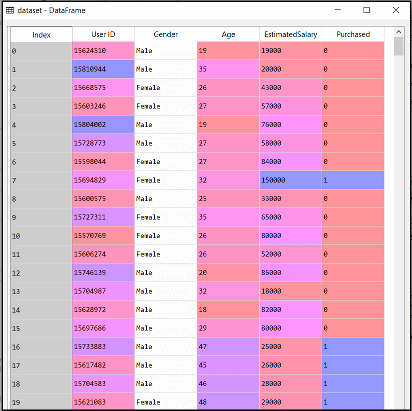
In the above code, we have loaded the dataset into our program using “dataset = pd.read_csv(‘user_data.csv’). The loaded dataset is divided into training and test set, and then we have scaled the feature variable.
The output for the dataset is given as:
2) Fitting Naive Bayes to the Training Set:
After the pre-processing step, now we will fit the Naive Bayes model to the Training set. Below is the code for it:
# Fitting Naive Bayes to the Training set
from sklearn.naive_bayes import GaussianNB
classifier = GaussianNB()
classifier.fit(x_train, y_train)
In the above code, we have used the GaussianNB classifier to fit it to the training dataset. We can also use other classifiers as per our requirement.
Output:
Out[6]: GaussianNB(priors=None, var_smoothing=1e-09)
3) Prediction of the test set result:
Now we will predict the test set result. For this, we will create a new predictor variable y_pred, and will use the predict function to make the predictions.
# Predicting the Test set results
y_pred = classifier.predict(x_test)
Output:
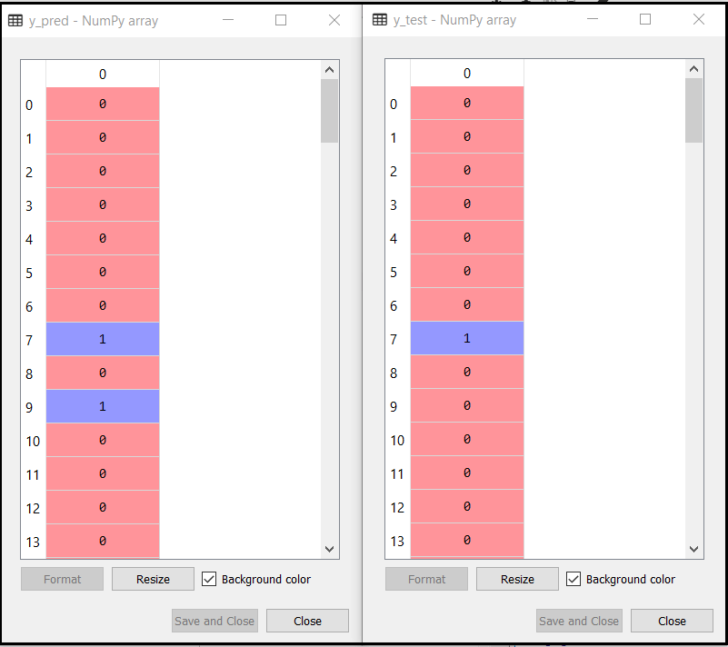
The above output shows the result for prediction vector y_pred and real vector y_test. We can see that some predications are different from the real values, which are the incorrect predictions.
4) Creating Confusion Matrix:
Now we will check the accuracy of the Naive Bayes classifier using the Confusion matrix. Below is the code for it:
# Making the Confusion Matrix
from sklearn.metrics import confusion_matrix
cm = confusion_matrix(y_test, y_pred)
Output:
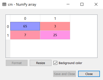
As we can see in the above confusion matrix output, there are 7+3= 10 incorrect predictions, and 65+25=90 correct predictions.
5) Visualizing the training set result:
Next we will visualize the training set result using Naïve Bayes Classifier. Below is the code for it:
# Visualising the Training set results
from matplotlib.colors import ListedColormap
x_set, y_set = x_train, y_train
X1, X2 = nm.meshgrid(nm.arange(start = x_set[:, 0].min() - 1, stop = x_set[:, 0].max() + 1, step = 0.01),
                     nm.arange(start = x_set[:, 1].min() - 1, stop = x_set[:, 1].max() + 1, step = 0.01))
mtp.contourf(X1, X2, classifier.predict(nm.array([X1.ravel(), X2.ravel()]).T).reshape(X1.shape),
             alpha = 0.75, cmap = ListedColormap(('purple', 'green')))
mtp.xlim(X1.min(), X1.max())
mtp.ylim(X2.min(), X2.max())
for i, j in enumerate(nm.unique(y_set)):
    mtp.scatter(x_set[y_set == j, 0], x_set[y_set == j, 1],
                c = ListedColormap(('purple', 'green'))(i), label = j)
mtp.title('Naive Bayes (Training set)')
mtp.xlabel('Age')
mtp.ylabel('Estimated Salary')
mtp.legend()
mtp.show()
Output:
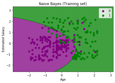
In the above output we can see that the Naïve Bayes classifier has segregated the data points with the fine boundary. It is Gaussian curve as we have used GaussianNB classifier in our code.
6) Visualizing the Test set result:
# Visualising the Test set results
from matplotlib.colors import ListedColormap
x_set, y_set = x_test, y_test
X1, X2 = nm.meshgrid(nm.arange(start = x_set[:, 0].min() - 1, stop = x_set[:, 0].max() + 1, step = 0.01),
                     nm.arange(start = x_set[:, 1].min() - 1, stop = x_set[:, 1].max() + 1, step = 0.01))
mtp.contourf(X1, X2, classifier.predict(nm.array([X1.ravel(), X2.ravel()]).T).reshape(X1.shape),
             alpha = 0.75, cmap = ListedColormap(('purple', 'green')))
mtp.xlim(X1.min(), X1.max())
mtp.ylim(X2.min(), X2.max())
for i, j in enumerate(nm.unique(y_set)):
    mtp.scatter(x_set[y_set == j, 0], x_set[y_set == j, 1],
                c = ListedColormap(('purple', 'green'))(i), label = j)
mtp.title('Naive Bayes (test set)')
mtp.xlabel('Age')
mtp.ylabel('Estimated Salary')
mtp.legend()
mtp.show()
Output:
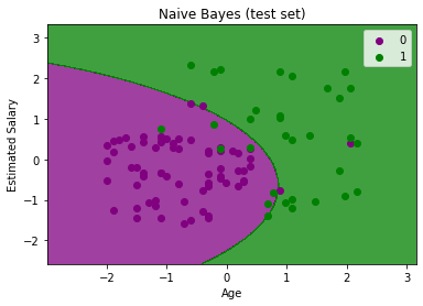
The above output is final output for test set data. As we can see the classifier has created a Gaussian curve to divide the “purchased” and “not purchased” variables. There are some wrong predictions which we have calculated in Confusion matrix. But still it is pretty good classifier.