
The Pearson’s Chi-Square statistical hypothesis is a test for independence between categorical variables. In this article, we will perform the test using a mathematical approach and then using Python’s SciPy module.
First, let us see the mathematical approach :
The Contingency Table :
A Contingency table (also called crosstab) is used in statistics to summarise the relationship between several categorical variables. Here, we take a table that shows the number of men and women buying different types of pets.
| dog | cat | bird | total | |
| men | 207 | 282 | 241 | 730 |
| women | 234 | 242 | 232 | 708 |
| total | 441 | 524 | 473 | 1438 |
The aim of the test is to conclude whether the two variables( gender and choice of pet ) are related to each other.
Null hypothesis:
We start by defining the null hypothesis (H0) which states that there is no relation between the variables. An alternate hypothesis would state that there is a significant relation between the two.
We can verify the hypothesis by these methods:
- Using p-value:
We define a significance factor to determine whether the relation between the variables is of considerable significance. Generally a significance factor or alpha value of 0.05 is chosen. This alpha value denotes the probability of erroneously rejecting H0 when it is true. A lower alpha value is chosen in cases where we expect more precision. If the p-value for the test comes out to be strictly greater than the alpha value, then H0 holds true.
- Using chi-square value:
If our calculated value of chi-square is less or equal to the tabular(also called critical) value of chi-square, then H0 holds true.
Expected Values Table :
Next, we prepare a similar table of calculated(or expected) values. To do this we need to calculate each item in the new table as :

The expected values table :
| dog | cat | bird | total | |
| men | 223.87343533 | 266.00834492 | 240.11821975 | 730 |
| women | 217.12656467 | 257.99165508 | 232.88178025 | 708 |
| total | 441 | 524 | 473 | 1438 |
Chi-Square Table :
We prepare this table by calculating for each item the following:

The chi-square table:
| observed (o) | calculated (c) | (o-c)^2 / c | |
| 207 | 223.87343533 | 1.2717579435607573 | |
| 282 | 266.00834492 | 0.9613722161954465 | |
| 241 | 240.11821975 | 0.003238139990850831 | |
| 234 | 217.12656467 | 1.3112758457617977 | |
| 242 | 257.99165508 | 0.991245364156322 | |
| 232 | 232.88178025 | 0.0033387601600580606 | |
| Total | 4.542228269825232 |
From this table, we obtain the total of the last column, which gives us the calculated value of chi-square. Hence the calculated value of chi-square is 4.542228269825232
Now, we need to find the critical value of chi-square. We can obtain this from a table. To use this table, we need to know the degrees of freedom for the dataset. The degrees of freedom is defined as : (no. of rows – 1) * (no. of columns – 1).
Hence, the degrees of freedom is (2-1) * (3-1) = 2
Now, let us look at the table and find the value corresponding to 2 degrees of freedom and 0.05 significance factor :
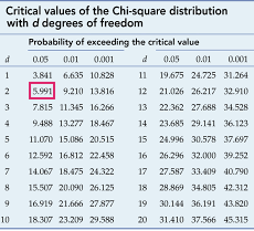
The tabular or critical value of chi-square here is 5.991
Hence, pip install scipy
The chi2_contingency() function of scipy.stats module takes as input, the contingency table in 2d array format. It returns a tuple containing test statistics, the p-value, degrees of freedom and expected table(the one we created from the calculated values) in that order.
Hence, we need to compare the obtained p-value with alpha value of 0.05.
from scipy.stats import chi2_contingency

# defining the table
data = [[207, 282, 241], [234, 242, 232]]
stat, p, dof, expected = chi2_contingency(data)

# interpret p-value
alpha = 0.05
print("p value is " + str(p))
if p <= alpha:
    print('Dependent (reject H0)')
else:
    print('Independent (H0 holds true)')
Output :
p value is 0.1031971404730939
Independent (H0 holds true)
Since,
p-value > alpha
Therefore, we accept H0, that is, the variables do not have a significant relation.