SVM Kernels
In practice, SVM algorithm is implemented with kernel that transforms an input data space into the required form. SVM uses a technique called the kernel trick in which kernel takes a low dimensional input space and transforms it into a higher dimensional space. In simple words, kernel converts non-separable problems into separable problems by adding more dimensions to it. It makes SVM more powerful, flexible and accurate. The following are some of the types of kernels used by SVM −
Linear Kernel
It can be used as a dot product between any two observations. The formula of linear kernel is as below −
k(x,xi) = sum(x*xi)
From the above formula, we can see that the product between two vectors say 𝑥 & 𝑥𝑖 is the sum of the multiplication of each pair of input values.
Polynomial Kernel
It is more generalized form of linear kernel and distinguish curved or nonlinear input space. Following is the formula for polynomial kernel −
K(x, xi) = 1 + sum(x * xi)^d
Here d is the degree of polynomial, which we need to specify manually in the learning algorithm.
Radial Basis Function (RBF) Kernel
RBF kernel, mostly used in SVM classification, maps input space in indefinite dimensional space. Following formula explains it mathematically −
K(x,xi) = exp(-gamma * sum((x – xi^2))
Here, gamma ranges from 0 to 1. We need to manually specify it in the learning algorithm. A good default value of gamma is 0.1.
As we implemented SVM for linearly separable data, we can implement it in Python for the data that is not linearly separable. It can be done by using kernels.
Example
The following is an example for creating an SVM classifier by using kernels. We will be using iris dataset from scikit-learn −
We will start by importing following packages −
import pandas as pd
import numpy as np
from sklearn import svm, datasets
import matplotlib.pyplot as plt
Now, we need to load the input data −
iris = datasets.load_iris()
From this dataset, we are taking first two features as follows −
X = iris.data[:, :2]
y = iris.target
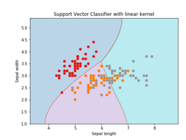
Next, we will plot the SVM boundaries with original data as follows −
x_min, x_max = X[:, 0].min() - 1, X[:, 0].max() + 1
y_min, y_max = X[:, 1].min() - 1, X[:, 1].max() + 1
h = (x_max / x_min)/100
xx, yy = np.meshgrid(np.arange(x_min, x_max, h),
   np.arange(y_min, y_max, h))
X_plot = np.c_[xx.ravel(), yy.ravel()]
Now, we need to provide the value of regularization parameter as follows −
C = 1.0
Next, SVM classifier object can be created as follows −
Svc_classifier = svm.SVC(kernel=’linear’, C=C).fit(X, y)
Z = svc_classifier.predict(X_plot)
Z = Z.reshape(xx.shape)
plt.figure(figsize=(15, 5))
plt.subplot(121)
plt.contourf(xx, yy, Z, cmap=plt.cm.tab10, alpha=0.3)
plt.scatter(X[:, 0], X[:, 1], c=y, cmap=plt.cm.Set1)
plt.xlabel('Sepal length')
plt.ylabel('Sepal width')
plt.xlim(xx.min(), xx.max())
plt.title('Support Vector Classifier with linear kernel')
Output
Text(0.5, 1.0, 'Support Vector Classifier with linear kernel')

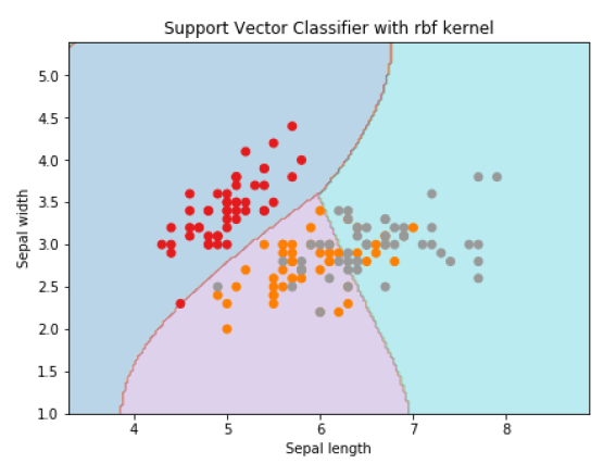
For creating SVM classifier with rbf kernel, we can change the kernel to rbf as follows −
Svc_classifier = svm.SVC(kernel='rbf', gamma =‘auto’,C=C).fit(X, y)
Z = svc_classifier.predict(X_plot)
Z = Z.reshape(xx.shape)
plt.figure(figsize=(15, 5))
plt.subplot(121)
plt.contourf(xx, yy, Z, cmap=plt.cm.tab10, alpha=0.3)
plt.scatter(X[:, 0], X[:, 1], c=y, cmap=plt.cm.Set1)
plt.xlabel('Sepal length')
plt.ylabel('Sepal width')
plt.xlim(xx.min(), xx.max())
plt.title('Support Vector Classifier with rbf kernel')
Output
Text(0.5, 1.0, 'Support Vector Classifier with rbf kernel')

We put the value of gamma to ‘auto’ but you can provide its value between 0 to 1 also.
