Regression in Supervised Learning

Regression models are used to predict a continuous value. Predicting prices of a house given the features of house like size, price etc is one of the common examples of Regression. It is a supervised technique. A detailed explanation on types of Machine Learning and some important concepts is given in my previous article.

Types of Regression

Simple Linear Regression
Polynomial Regression
Support Vector Regression
Decision Tree Regression
Random Forest Regression

Simple Linear Regression

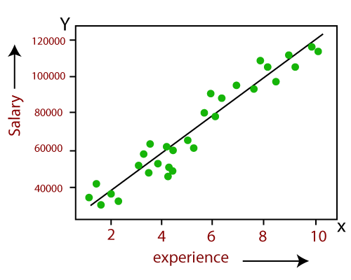
This is one of the most common and interesting type of Regression technique. Here we predict a target variable Y based on the input variable X. A linear relationship should exist between target variable and predictor and so comes the name Linear Regression.

Consider predicting the salary of an employee based on his/her age. We can easily identify that there seems to be a correlation between employee’s age and salary (more the age more is the salary). The hypothesis of linear regression is

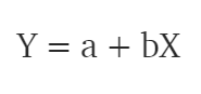
Y represents salary, X is employee’s age and a and b are the coefficients of the equation. So in order to predict Y (salary) given X (age), we need to know the values of a and b (the model’s coefficients).

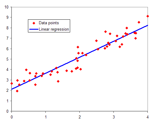
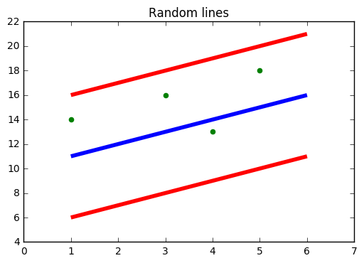
While training and building a regression model, it is these coefficients which are learned and fitted to training data. The aim of the training is to find the best fit line such that cost function is minimized. The cost function helps in measuring the error. During the training process, we try to minimize the error between actual and predicted values and thus minimizing the cost function.

In the figure, the red points are the data points and the blue line is the predicted line for the training data. To get the predicted value, these data points are projected on to the line.

To summarize, our aim is to find such values of coefficients which will minimize the cost function. The most common cost function is Mean Squared Error (MSE) which is equal to the average squared difference between an observation’s actual and predicted values. The coefficient values can be calculated using the Gradient Descent approach which will be discussed in detail in later articles. To give a brief understanding, in Gradient descent we start with some random values of coefficients, compute the gradient of cost function on these values, update the coefficients and calculate the cost function again. This process is repeated until we find a minimum value of cost function.

Polynomial Regression

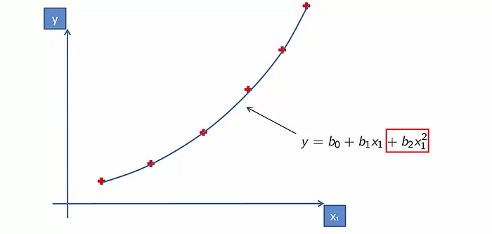
In polynomial regression, we transform the original features into polynomial features of a given degree and then apply Linear Regression on it. Consider the above linear model Y = a+bX is transformed into something like

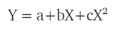
It is still a linear model but the curve is now quadratic rather than a line. Scikit-Learn provides PolynomialFeatures class to transform the features.

If we increase the degree to a very high value, the curve becomes overfitted as it learns the noise in the data as well.

Support Vector Regression

In SVR, we identify a hyperplane with maximum margin such that the maximum number of data points are within that margin. SVRs are almost similar to the SVM classification algorithm. We will discuss the SVM algorithm in detail in my next article.

Instead of minimizing the error rate as in simple linear regression, we try to fit the error within a certain threshold. Our objective in SVR is to basically consider the points that are within the margin. Our best fit line is the hyperplane that has the maximum number of points.

Decision Tree Regression

Decision trees can be used for classification as well as regression. In decision trees, at each level, we need to identify the splitting attribute. In the case of regression, the ID3 algorithm can be used to identify the splitting node by reducing the standard deviation (in classification information gain is used).

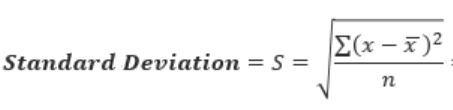
A decision tree is built by partitioning the data into subsets containing instances with similar values (homogenous). Standard deviation is used to calculate the homogeneity of a numerical sample. If the numerical sample is completely homogeneous, its standard deviation is zero.

The steps for finding the splitting node is briefly described below:

Calculate the standard deviation of the target variable using below formula.

2. Split the dataset on different attributes and calculate the standard deviation for each branch (standard deviation for target and predictor). This value is subtracted from the standard deviation before the split. The result is the standard deviation reduction.

3. The attribute with the largest standard deviation reduction is chosen as the splitting node.

4. The dataset is divided based on the values of the selected attribute. This process is run recursively on the non-leaf branches until all data is processed.

To avoid overfitting, the Coefficient of Deviation (CV) is used which decides when to stop branching. Finally, the average of each branch is assigned to the related leaf node (in regression mean is taken whereas in classification mode of leaf nodes is taken).

Random Forest Regression

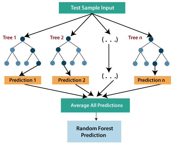
Random forest is an ensemble approach where we take into account the predictions of several decision regression trees.

Select K random points
Identify n where n is the number of decision tree regressors to be created. Repeat steps 1 and 2 to create several regression trees.
The average of each branch is assigned to the leaf node in each decision tree.
To predict output for a variable, the average of all the predictions of all decision trees are taken into consideration.

Random Forest prevents overfitting (which is common in decision trees) by creating random subsets of the features and building smaller trees using these subsets.

Regression analysis is a statistical method to model the relationship between a dependent (target) and independent (predictor) variables with one or more independent variables. More specifically, Regression analysis helps us to understand how the value of the dependent variable is changing corresponding to an independent variable when other independent variables are held fixed. It predicts continuous/real values such as temperature, age, salary, price, etc.

We can understand the concept of regression analysis using the below example:

Example: Suppose there is a marketing company A, who does various advertisement every year and get sales on that. The below list shows the advertisement made by the company in the last 5 years and the corresponding sales:

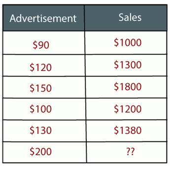
Now, the company wants to do the advertisement of $200 in the year 2019 and wants to know the prediction about the sales for this year. So to solve such type of prediction problems in machine learning, we need regression analysis.9.1M209Exception Handling in Java – Javatpoint

Regression is a supervised learning technique which helps in finding the correlation between variables and enables us to predict the continuous output variable based on the one or more predictor variables. It is mainly used for prediction, forecasting, time series modeling, and determining the causal-effect relationship between variables.

In Regression, we plot a graph between the variables which best fits the given datapoints, using this plot, the machine learning model can make predictions about the data. In simple words, “Regression shows a line or curve that passes through all the datapoints on target-predictor graph in such a way that the vertical distance between the datapoints and the regression line is minimum.” The distance between datapoints and line tells whether a model has captured a strong relationship or not.

Some examples of regression can be as:

Prediction of rain using temperature and other factors
Determining Market trends
Prediction of road accidents due to rash driving.

Terminologies Related to the Regression Analysis:

Dependent Variable: The main factor in Regression analysis which we want to predict or understand is called the dependent variable. It is also called target variable.
Independent Variable: The factors which affect the dependent variables or which are used to predict the values of the dependent variables are called independent variable, also called as a predictor.
Outliers: Outlier is an observation which contains either very low value or very high value in comparison to other observed values. An outlier may hamper the result, so it should be avoided.
Multicollinearity: If the independent variables are highly correlated with each other than other variables, then such condition is called Multicollinearity. It should not be present in the dataset, because it creates problem while ranking the most affecting variable.
Underfitting and Overfitting: If our algorithm works well with the training dataset but not well with test dataset, then such problem is called Overfitting. And if our algorithm does not perform well even with training dataset, then such problem is called underfitting.

Why do we use Regression Analysis?

As mentioned above, Regression analysis helps in the prediction of a continuous variable. There are various scenarios in the real world where we need some future predictions such as weather condition, sales prediction, marketing trends, etc., for such case we need some technology which can make predictions more accurately. So for such case we need Regression analysis which is a statistical method and used in machine learning and data science. Below are some other reasons for using Regression analysis:

Regression estimates the relationship between the target and the independent variable.
It is used to find the trends in data.
It helps to predict real/continuous values.
By performing the regression, we can confidently determine the most important factor, the least important factor, and how each factor is affecting the other factors.

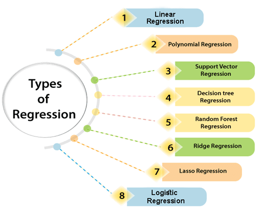
Types of Regression

There are various types of regressions which are used in data science and machine learning. Each type has its own importance on different scenarios, but at the core, all the regression methods analyze the effect of the independent variable on dependent variables. Here we are discussing some important types of regression which are given below:

Linear Regression
Logistic Regression
Polynomial Regression
Support Vector Regression
Decision Tree Regression
Random Forest Regression
Ridge Regression
Lasso Regression:

Linear Regression:

Linear regression is a statistical regression method which is used for predictive analysis.
It is one of the very simple and easy algorithms which works on regression and shows the relationship between the continuous variables.
It is used for solving the regression problem in machine learning.
Linear regression shows the linear relationship between the independent variable (X-axis) and the dependent variable (Y-axis), hence called linear regression.
If there is only one input variable (x), then such linear regression is called simple linear regression. And if there is more than one input variable, then such linear regression is called multiple linear regression.
The relationship between variables in the linear regression model can be explained using the below image. Here we are predicting the salary of an employee on the basis of the year of experience.

Below is the mathematical equation for Linear regression:

Y= aX+b

Here, Y = dependent variables (target variables),
X= Independent variables (predictor variables),
a and b are the linear coefficients

Some popular applications of linear regression are:

Analyzing trends and sales estimates
Salary forecasting
Real estate prediction
Arriving at ETAs in traffic.

Logistic Regression:

Logistic regression is another supervised learning algorithm which is used to solve the classification problems. In classification problems, we have dependent variables in a binary or discrete format such as 0 or 1.
Logistic regression algorithm works with the categorical variable such as 0 or 1, Yes or No, True or False, Spam or not spam, etc.
It is a predictive analysis algorithm which works on the concept of probability.
Logistic regression is a type of regression, but it is different from the linear regression algorithm in the term how they are used.
Logistic regression uses sigmoid function or logistic function which is a complex cost function. This sigmoid function is used to model the data in logistic regression. The function can be represented as:

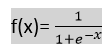
f(x)= Output between the 0 and 1 value.
x= input to the function
e= base of natural logarithm.

When we provide the input values (data) to the function, it gives the S-curve as follows:

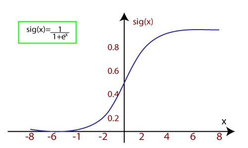
It uses the concept of threshold levels, values above the threshold level are rounded up to 1, and values below the threshold level are rounded up to 0.

There are three types of logistic regression:

Binary(0/1, pass/fail)
Multi(cats, dogs, lions)
Ordinal(low, medium, high)

Polynomial Regression:

Polynomial Regression is a type of regression which models the non-linear dataset using a linear model.
It is similar to multiple linear regression, but it fits a non-linear curve between the value of x and corresponding conditional values of y.
Suppose there is a dataset which consists of datapoints which are present in a non-linear fashion, so for such case, linear regression will not best fit to those datapoints. To cover such datapoints, we need Polynomial regression.
In Polynomial regression, the original features are transformed into polynomial features of given degree and then modeled using a linear model. Which means the datapoints are best fitted using a polynomial line.

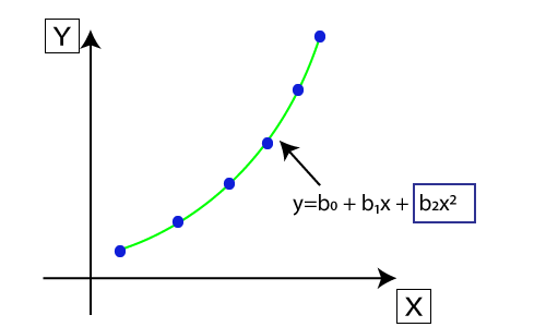
The equation for polynomial regression also derived from linear regression equation that means Linear regression equation Y= b₀+ b₁x, is transformed into Polynomial regression equation Y= b₀+b₁x+ b₂x²+ b₃x³+…..+ b_nxⁿ.
Here Y is the predicted/target output, b₀, b₁,… b_n are the regression coefficients. x is our independent/input variable.
The model is still linear as the coefficients are still linear with quadratic

Note: This is different from Multiple Linear regression in such a way that in Polynomial regression, a single element has different degrees instead of multiple variables with the same degree.

Support Vector Regression:

Support Vector Machine is a supervised learning algorithm which can be used for regression as well as classification problems. So if we use it for regression problems, then it is termed as Support Vector Regression.

Support Vector Regression is a regression algorithm which works for continuous variables. Below are some keywords which are used in Support Vector Regression:

Kernel: It is a function used to map a lower-dimensional data into higher dimensional data.
Hyperplane: In general SVM, it is a separation line between two classes, but in SVR, it is a line which helps to predict the continuous variables and cover most of the datapoints.
Boundary line: Boundary lines are the two lines apart from hyperplane, which creates a margin for datapoints.
Support vectors: Support vectors are the datapoints which are nearest to the hyperplane and opposite class.

In SVR, we always try to determine a hyperplane with a maximum margin, so that maximum number of datapoints are covered in that margin. The main goal of SVR is to consider the maximum datapoints within the boundary lines and the hyperplane (best-fit line) must contain a maximum number of datapoints. Consider the below image:

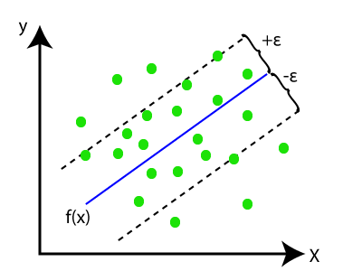
Here, the blue line is called hyperplane, and the other two lines are known as boundary lines.

Decision Tree Regression:

Decision Tree is a supervised learning algorithm which can be used for solving both classification and regression problems.
It can solve problems for both categorical and numerical data
Decision Tree regression builds a tree-like structure in which each internal node represents the “test” for an attribute, each branch represent the result of the test, and each leaf node represents the final decision or result.
A decision tree is constructed starting from the root node/parent node (dataset), which splits into left and right child nodes (subsets of dataset). These child nodes are further divided into their children node, and themselves become the parent node of those nodes. Consider the below image:

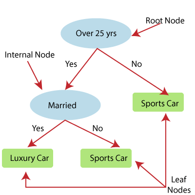
Above image showing the example of Decision Tee regression, here, the model is trying to predict the choice of a person between Sports cars or Luxury car.

Random forest is one of the most powerful supervised learning algorithms which is capable of performing regression as well as classification tasks.
The Random Forest regression is an ensemble learning method which combines multiple decision trees and predicts the final output based on the average of each tree output. The combined decision trees are called as base models, and it can be represented more formally as:

g(x)= f₀(x)+ f₁(x)+ f₂(x)+....

Random forest uses Bagging or Bootstrap Aggregation technique of ensemble learning in which aggregated decision tree runs in parallel and do not interact with each other.
With the help of Random Forest regression, we can prevent Overfitting in the model by creating random subsets of the dataset.

Ridge Regression:

Ridge regression is one of the most robust versions of linear regression in which a small amount of bias is introduced so that we can get better long term predictions.
The amount of bias added to the model is known as Ridge Regression penalty. We can compute this penalty term by multiplying with the lambda to the squared weight of each individual features.
The equation for ridge regression will be:

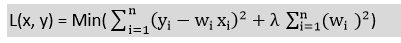
A general linear or polynomial regression will fail if there is high collinearity between the independent variables, so to solve such problems, Ridge regression can be used.
Ridge regression is a regularization technique, which is used to reduce the complexity of the model. It is also called as L2 regularization.
It helps to solve the problems if we have more parameters than samples.

Lasso Regression:

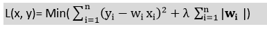
Lasso regression is another regularization technique to reduce the complexity of the model.
It is similar to the Ridge Regression except that penalty term contains only the absolute weights instead of a square of weights.
Since it takes absolute values, hence, it can shrink the slope to 0, whereas Ridge Regression can only shrink it near to 0.
It is also called as L1 regularization. The equation for Lasso regression will be: