
Now we will implement the Decision tree using Python. For this, we will use the dataset “user_data.csv,” which we have used in previous classification models. By using the same dataset, we can compare the Decision tree classifier with other classification models such as KNN SVM, Logistic Regression, etc.
Steps will also remain the same, which are given below:
- Data Pre-processing step
- Fitting a Decision-Tree algorithm to the Training set
- Predicting the test result
- Test accuracy of the result(Creation of Confusion matrix)
- Visualizing the test set result.
1. Data Pre-Processing Step:
Below is the code for the pre-processing step:
# importing libraries
import numpy as nm
import matplotlib.pyplot as mtp
import pandas as pd

#importing datasets
data_set= pd.read_csv('user_data.csv')

#Extracting Independent and dependent Variable
x= data_set.iloc[:, [2,3]].values
y= data_set.iloc[:, 4].values

# Splitting the dataset into training and test set.
from sklearn.model_selection import train_test_split
x_train, x_test, y_train, y_test= train_test_split(x, y, test_size= 0.25, random_state=0)

#feature Scaling
from sklearn.preprocessing import StandardScaler
st_x= StandardScaler()
x_train= st_x.fit_transform(x_train)
x_test= st_x.transform(x_test)
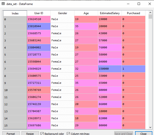
In the above code, we have pre-processed the data. Where we have loaded the dataset, which is given as:
2. Fitting a Decision-Tree algorithm to the Training set
Now we will fit the model to the training set. For this, we will import the DecisionTreeClassifier class from sklearn.tree library. Below is the code for it:
#Fitting Decision Tree classifier to the training set
From sklearn.tree import DecisionTreeClassifier
classifier= DecisionTreeClassifier(criterion='entropy', random_state=0)
classifier.fit(x_train, y_train)
In the above code, we have created a classifier object, in which we have passed two main parameters;
- “criterion=’entropy’: Criterion is used to measure the quality of split, which is calculated by information gain given by entropy.
- random_state=0″: For generating the random states.
Below is the output for this:
Out[8]:
DecisionTreeClassifier(class_weight=None, criterion='entropy', max_depth=None,
max_features=None, max_leaf_nodes=None,
min_impurity_decrease=0.0, min_impurity_split=None,
min_samples_leaf=1, min_samples_split=2,
min_weight_fraction_leaf=0.0, presort=False,
                       random_state=0, splitter='best')
3. Predicting the test result
Now we will predict the test set result. We will create a new prediction vector y_pred. Below is the code for it:
#Predicting the test set result
y_pred= classifier.predict(x_test)
Output:
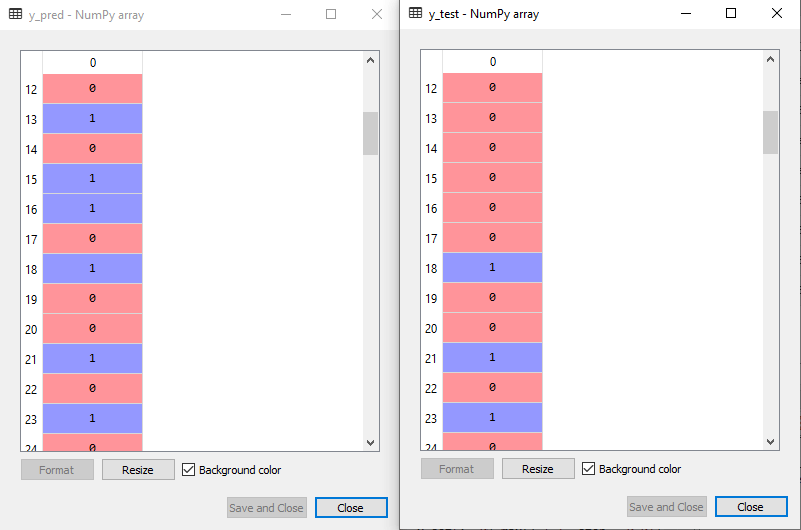
In the below output image, the predicted output and real test output are given. We can clearly see that there are some values in the prediction vector, which are different from the real vector values. These are prediction errors.
4. Test accuracy of the result (Creation of Confusion matrix)
In the above output, we have seen that there were some incorrect predictions, so if we want to know the number of correct and incorrect predictions, we need to use the confusion matrix. Below is the code for it:
#Creating the Confusion matrix
from sklearn.metrics import confusion_matrix
cm= confusion_matrix(y_test, y_pred)
Output:
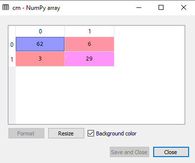
In the above output image, we can see the confusion matrix, which has 6+3= 9 incorrect predictions and62+29=91 correct predictions. Therefore, we can say that compared to other classification models, the Decision Tree classifier made a good prediction.
5. Visualizing the training set result:
Here we will visualize the training set result. To visualize the training set result we will plot a graph for the decision tree classifier. The classifier will predict yes or No for the users who have either Purchased or Not purchased the SUV car as we did in Logistic Regression. Below is the code for it:
#Visulaizing the trianing set result
from matplotlib.colors import ListedColormap
x_set, y_set = x_train, y_train
x1, x2 = nm.meshgrid(nm.arange(start = x_set[:, 0].min() - 1, stop = x_set[:, 0].max() + 1, step  =0.01),
nm.arange(start = x_set[:, 1].min() - 1, stop = x_set[:, 1].max() + 1, step = 0.01))
mtp.contourf(x1, x2, classifier.predict(nm.array([x1.ravel(), x2.ravel()]).T).reshape(x1.shape),
alpha = 0.75, cmap = ListedColormap(('purple','green' )))
mtp.xlim(x1.min(), x1.max())
mtp.ylim(x2.min(), x2.max())
fori, j in enumerate(nm.unique(y_set)):
mtp.scatter(x_set[y_set == j, 0], x_set[y_set == j, 1],
        c = ListedColormap(('purple', 'green'))(i), label = j)
mtp.title('Decision Tree Algorithm (Training set)')
mtp.xlabel('Age')
mtp.ylabel('Estimated Salary')
mtp.legend()
mtp.show()
Output:
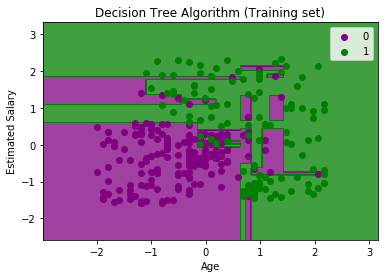
The above output is completely different from the rest classification models. It has both vertical and horizontal lines that are splitting the dataset according to the age and estimated salary variable.
As we can see, the tree is trying to capture each dataset, which is the case of overfitting.
6. Visualizing the test set result:
Visualization of test set result will be similar to the visualization of the training set except that the training set will be replaced with the test set.
#Visulaizing the test set result
from matplotlib.colors import ListedColormap
x_set, y_set = x_test, y_test
x1, x2 = nm.meshgrid(nm.arange(start = x_set[:, 0].min() - 1, stop = x_set[:, 0].max() + 1, step  =0.01),
nm.arange(start = x_set[:, 1].min() - 1, stop = x_set[:, 1].max() + 1, step = 0.01))
mtp.contourf(x1, x2, classifier.predict(nm.array([x1.ravel(), x2.ravel()]).T).reshape(x1.shape),
alpha = 0.75, cmap = ListedColormap(('purple','green' )))
mtp.xlim(x1.min(), x1.max())
mtp.ylim(x2.min(), x2.max())
fori, j in enumerate(nm.unique(y_set)):
mtp.scatter(x_set[y_set == j, 0], x_set[y_set == j, 1],
        c = ListedColormap(('purple', 'green'))(i), label = j)
mtp.title('Decision Tree Algorithm(Test set)')
mtp.xlabel('Age')
mtp.ylabel('Estimated Salary')
mtp.legend()
mtp.show()
Output:
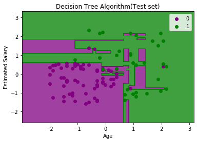
As we can see in the above image that there are some green data points within the purple region and vice versa. So, these are the incorrect predictions which we have discussed in the confusion matrix.