
Housing prices are an important reflection of the economy, and housing price ranges are of great interest for both buyers and sellers. Ask a home buyer to describe their dream house, and they probably won’t begin with the height of the basement ceiling or the proximity to an east-west railroad. But this playground competition’s data-set proves that much more influences price negotiations than the number of bedrooms or a white-picket fence.
About the Dataset
Housing prices are an important reflection of the economy, and housing price ranges are of great interest for both buyers and sellers. In this project, house prices will be predicted given explanatory variables that cover many aspects of residential houses. The goal of this project is to create a regression model that is able to accurately estimate the price of the house given the features.
In this dataset made for predicting the Boston House Price Prediction. Here I just show the all of the feature for each house separately. Such as Number of Rooms, Crime rate of the House’s Area and so on. We’ll show in the upcoming part.
Data Overview

1. CRIM per capital crime rate by town
2. ZN proportion of residential land zoned for lots over 25,000 sq.ft.
3. INDUS proportion of non-retail business acres per town
4. CHAS Charles River dummy variable (= 1 if tract bounds river; 0 otherwise)
5. NOX nitric oxides concentration (parts per 10 million)
6. RM average number of rooms per dwelling
7. AGE proportion of owner-occupied units built prior to 1940
8. DIS weighted distances to five Boston employment centers
9. RAD index of accessibility to radial highways
10.TAX full-value property-tax rate per 10,000 USD
11. PTRATIO pupil-teacher ratio by town
12. Black 1000(Bk — 0.63)² where Bk is the proportion of blacks by town
13. LSTAT % lower status of the population
About the Algorithms used in
The major aim of in this project is to predict the house prices based on the features using some of the regression techniques and algorithms.
1. Linear Regression
2. Random Forest Regressor
Machine Learning Packages are used for in this Project

Data Collection
I got the Dataset from Kaggle. This Dataset consist several features such as Number of Rooms, Crime Rate, and Tax and so on. Let’s know about how to read the dataset into the Jupyter Notebook. You can download the dataset from Kaggle in csv file format.
As well we can also able to get the dataset from the sklearn datasets. Yup! It’s available into the sklearn Dataset.
Let’s we see how can we retrieve the dataset from the sklearn dataset.
from sklearn.datasets import load_bostonX, y = load_boston(return_X_y=True)
Code for collecting data from CSV file into Jupyter Notebook!
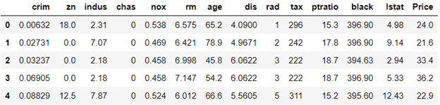
# Import librariesimport numpy as npimport pandas as pd# Import the datasetdf = pd.read_csv(“train.csv”)df.head()
Data Preprocessing
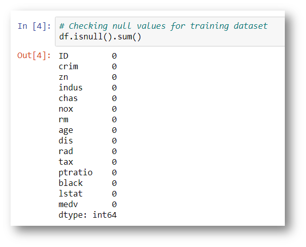
In this Boston Dataset we need not to clean the data. The dataset already cleaned when we download from the Kaggle. For your satisfaction i will show to number of null or missing values in the dataset. As well as we need to understand shape of the dataset.
# Shape of datasetprint(“Shape of Training dataset:”, df.shape)Shape of Training dataset: (333, 15)# Checking null values for training datasetdf.isnull().sum()
Note: The target variable is the last one which is called medv. So we can’t able to get confusion so I just rename the feature name medv into Price.
# Here lets change ‘medv’ column name to ‘Price’df.rename(columns={‘medv’:’Price’}, inplace=True)
Yup! Look that the feature or column name is changed!
Exploratory Data Analysis
In statistics, exploratory data analysis (EDA) is an approach to analyzing data sets to summarize their main characteristics, often with visual methods. A statistical model can be used or not, but primarily EDA is for seeing what the data can tell us beyond the formal modeling or hypothesis testing task.
# Information about the dataset featuresdf.info()

# Describedf.describe()

Feature Observation
# Finding out the correlation between the featurescorr = df.corr()corr.shape
First Understanding the correlation of features between target and other features
# Plotting the heatmap of correlation between featuresplt.figure(figsize=(14,14))sns.heatmap(corr, cbar=False, square= True, fmt=’.2%’, annot=True, cmap=’Greens’)

# Checking the null values using heatmap# There is any null values are occupyed heresns.heatmap(df.isnull(),yticklabels=False,cbar=False,cmap=’viridis’)
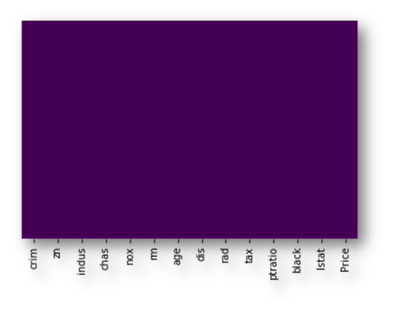
Note: There are no null or missing values here.
sns.set_style(‘whitegrid’)sns.countplot(x=’rad’,data=df)

sns.set_style(‘whitegrid’)sns.countplot(x=’chas’,data=df)

sns.set_style(‘whitegrid’)sns.countplot(x=’chas’,hue=’rad’,data=df,palette=’RdBu_r’)

sns.distplot(df[‘age’].dropna(),kde=False,color=’darkred’,bins=40)

sns.distplot(df[‘crim’].dropna(),kde=False,color=’darkorange’,bins=40)

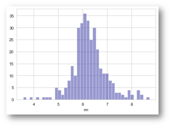
sns.distplot(df[‘rm’].dropna(),kde=False,color=’darkblue’,bins=40)
Feature Selection
Feature Selection is the process where you automatically or manually select those features which contribute most to your prediction variable or output in which you are interested in. Having irrelevant features in your data can decrease the accuracy of the models and make your model learn based on irrelevant features.
# Lets try to understand which are important feature for this datasetfrom sklearn.feature_selection import SelectKBestfrom sklearn.feature_selection import chi2X = df.iloc[:,0:13] #independent columnsy = df.iloc[:,-1] #target column i.e price range
Note: If we want to identify the best features for the target variables. We should make sure that the target variable should be int Values. That’s why I convert into the int value from the floating point value
y = np.round(df[‘Price’])#Apply SelectKBest class to extract top 5 best featuresbestfeatures = SelectKBest(score_func=chi2, k=5)fit = bestfeatures.fit(X,y)dfscores = pd.DataFrame(fit.scores_)dfcolumns = pd.DataFrame(X.columns)# Concat two dataframes for better visualizationfeatureScores = pd.concat([dfcolumns,dfscores],axis=1)featureScores.columns = [‘Specs’,’Score’] #naming the dataframe columnsfeatureScores
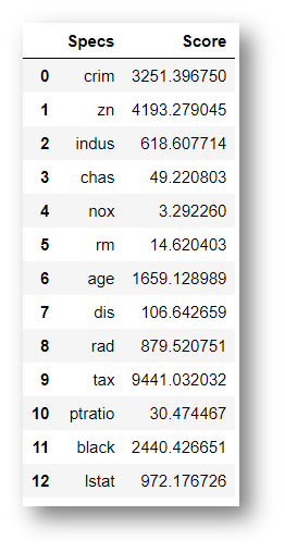
print(featureScores.nlargest(5,’Score’)) #print 5 best features
Index-Specs- Score
9 – tax -9441.032032
1- zn- 4193.279045
0 -crim- 3251.396750
11- black -2440.426651
6 -age -1659.128989
Feature Importance
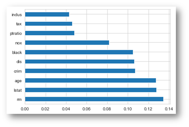
from sklearn.ensemble import ExtraTreesClassifierimport matplotlib.pyplot as pltmodel = ExtraTreesClassifier()model.fit(X,y)

print(model.feature_importances_) #use inbuilt class feature_importances of tree based classifiers
[0.11621392 0.02557494 0.03896227 0.01412571 0.07957026 0.12947365
0.11289525 0.10574315 0.04032395 0.05298918 0.04505287 0.10469546
0.13437938]
# Plot graph of feature importances for better visualizationfeat_importances = pd.Series(model.feature_importances_, index=X.columns)feat_importances.nlargest(10).plot(kind=’barh’)plt.show()
Model Fitting
Linear Regression


Random Forest Regressor


Prediction and Final Score:
Finally we made it!!!
Linear Regression
Model Score: 73.1% Accuracy
Training Accuracy: 72.9% Accuracy
Testing Accuracy: 73.1% Accuracy
Random Forest Regressor
Training Accuracy: 99.9% Accuracy.
Testing Accuracy: 99.8% Accuracy
Output & Conclusion

From the Exploratory Data Analysis, we could generate insight from the data. How each of the features relates to the target. Also, it can be seen from the evaluation of three models that Random Forest Regressor performed better than Linear Regression.